library(pruatlas)
library(dplyr)
#>
#> Attaching package: 'dplyr'
#> The following objects are masked from 'package:stats':
#>
#>     filter, lag
#> The following objects are masked from 'package:base':
#>
#>     intersect, setdiff, setequal, union
library(sf)
#> Linking to GEOS 3.11.0, GDAL 3.5.3, PROJ 9.1.0; sf_use_s2() is TRUE
library(ggplot2)
library(stringr)
library(readr)
library(purrr)
Single Country
FIR
Let’s plot Italian FIR at FL300
plot_country_fir("LI", "Italy", fl = 300)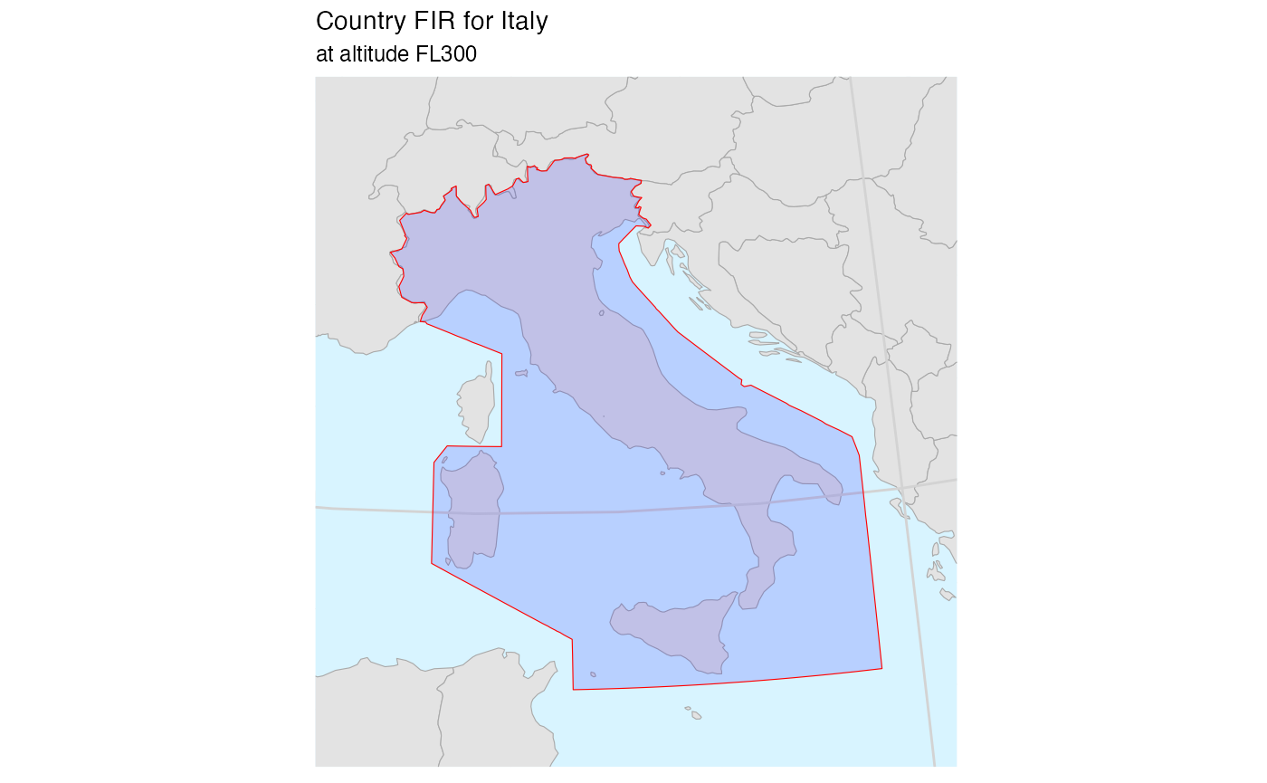
For UK, things are more complicated because it has also an Oceanic bit of volume
plot_country_fir("EG", "UK (oceanic)", fl = 200)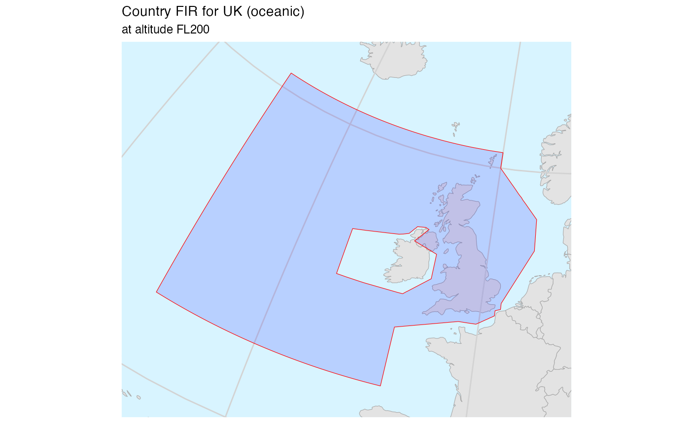
So to plot the continental part only we need to split things:
uk_continental <- firs_nm_406 %>%
  dplyr::filter(icao == "EG", min_fl <= 0, 0 <= max_fl) %>%
  dplyr::filter(!(id %in% c("EGGXFIR", "EGGX")))
plot_country_fir(
  "EG",
  "UK (continental)",
  firs = uk_continental,
  fl = 200)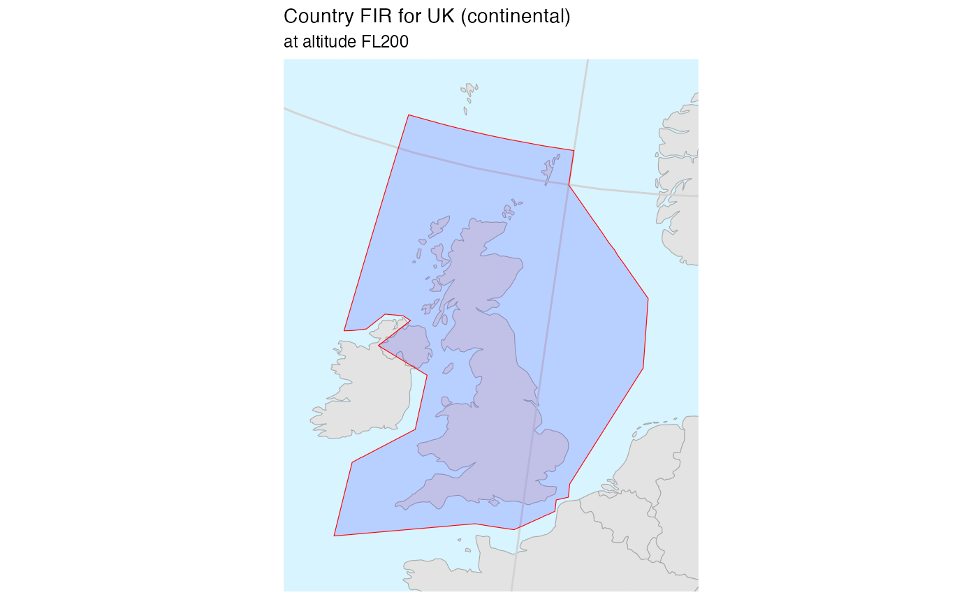
Aiport location in FIR
# some airports
apts <- tibble::tribble(
   ~ICAO_CODE, ~IATA_CODE,               ~LON,    ~LAT,           ~NAME,
       "EDDF",      "FRA",   8.5706, 50.0333,               "Frankfurt",
       "EHAM",      "AMS",   4.7642, 52.3080,               "Amsterdam",
       "LFPG",      "CDG",   2.5478, 49.0097, "Paris/Charles-De-Gaulle",
       "EGLL",      "LHR", -0.46139, 51.4775,         "London/Heathrow"
   )

# transform to sf
apts_sf <- apts %>%
   st_as_sf(coords = c("LON", "LAT"), crs = 4326)

# keep only EGLL
apt <- apts_sf %>%
      filter(ICAO_CODE == "EGLL")


# single country (FIR)
uk_continental <- firs_nm_406 %>%
   dplyr::filter(icao == "EG", min_fl <= 0, 0 <= max_fl) %>%
   dplyr::filter(!(id %in% c("EGGXFIR", "EGGX")))

bbox <- uk_continental %>%
   st_transform(crs = sf::st_crs(3035)) %>%
   st_bbox()

plot_country_fir(
  "EG",
  "UK (continental)",
  firs = uk_continental,
  fl = 200) +
  ggplot2::geom_sf(
    data = apt,
    shape = 10,
    size = 3) +
  ggplot2::geom_sf_text(
    data = apt,
    aes(label = ICAO_CODE),
    vjust = -0.5) +
  # (re-)zoom to the correct bounding box
  ggplot2::coord_sf(xlim = bbox[c(1, 3)], ylim = bbox[c(2, 4)]) +
  # (re-)define the title and subtitle (`plot_country_fir()` adds its own)
  ggtitle(label = str_glue("{name} ({icao})", name = apt$NAME, icao = apt$ICAO_CODE),
          subtitle = "United Kingdom FIR (continental) at FL200")
#> Coordinate system already present. Adding new coordinate system, which will
#> replace the existing one.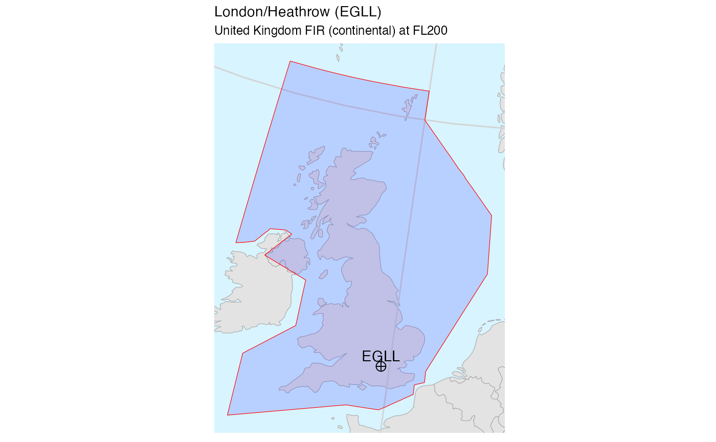
EUROCONTROL
Merged Member States FIRs
For plotting EUROCONTROL Member States’ FIR area we can select and merge the various airspaces:
plot_country_fir(icao_id = "E.|L.|UD|UG|GM|UK|GC",
                 "EUROCONTROL",
                 buffer = 350,
                 fl = 200)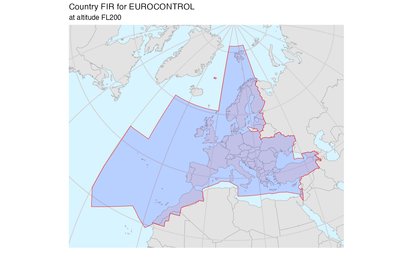
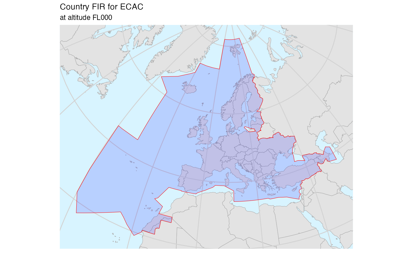
All Member States FIRs
ms_codes <- member_states %>%
  # filter out Germany (military, no specific FIR),
  #   Luxembourg (managed by Belgium) and Monaco (managed by France)
  filter(!icao %in% c("ET", "EL", "LN")) %>%
  distinct(icao) %>%
  pull(icao)


ms_firs <- ms_codes %>%
  purrr::map_dfr(~ suppressMessages(
    country_fir(pruatlas::firs_nm_406, icao_id = .x))) %>%
  mutate(id = str_sub(id, 1, 2)) %>%
  left_join(member_states %>%
              filter(!icao %in% c("ET", "EL", "LN")) %>%
              distinct(icao, .keep_all = TRUE),
            by = c("id" = "icao")) %>%
  mutate(
    name = case_when(
      id == "EB" ~ "Belgium and Luxemburg",
      id == "LF" ~ "France and Monaco",
      id == "LY" ~ "Serbia and Montenegro",
      id == "EG" ~ "United Kingdom",
      TRUE       ~ name),
    icao = id,
    min_fl = 200,
    max_fl = 200)

plot_country_fir(firs = ms_firs,
                 icao_id = ms_codes,
                 fl = 200,
                 name = "EUROCONTROL",
                 merge = FALSE)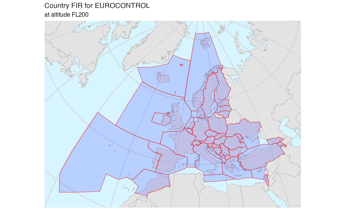
CRCO Charging Zones
You can get the CRCO charging zones boundaries from EUROCONTROL web site. This package stores a real file as an example.
bo <- system.file("extdata", "sbm_bz_20200527.txt", package = "pruatlas")
crco <- readr::read_lines(bo) %>%
  parse_airspace_crco() %>%
  mutate(icao = unit)
codes <- crco %>% pull(icao) %>% unique()

# country_fir(firs = crco,
#             icao_id = "E.|L.|UD|UG|GM|UK|GC",
#             fl = 200, merge = FALSE)
#
# ggplot(crco) + geom_sf()

plot_country_fir(firs = crco,
                 fl = 200,
                 icao_id = codes,
                 name = "CRCO charging zones",
                 merge = FALSE)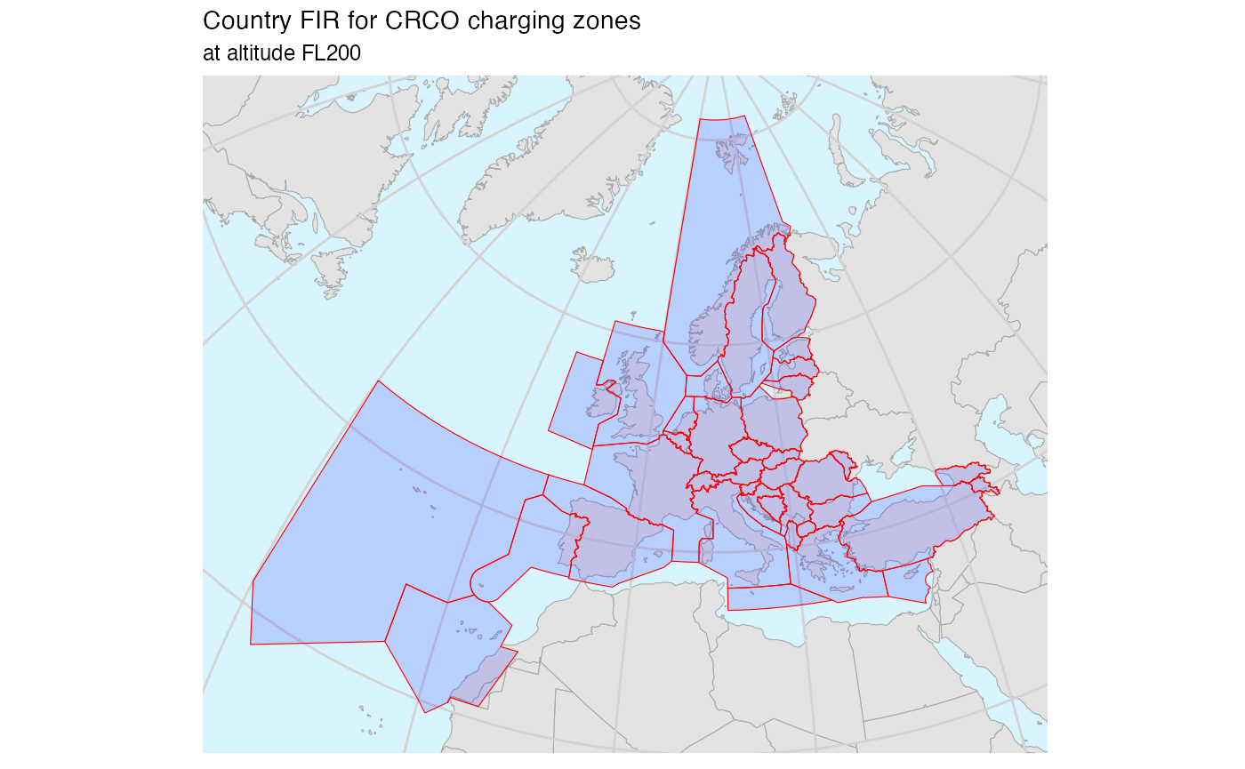
STATFOR Areas
ECAC North West
ecac_northwest() %>%
  plot_country_fir(icao_id = "ECNW",
                   name = "ECAC North West",
                   firs = .)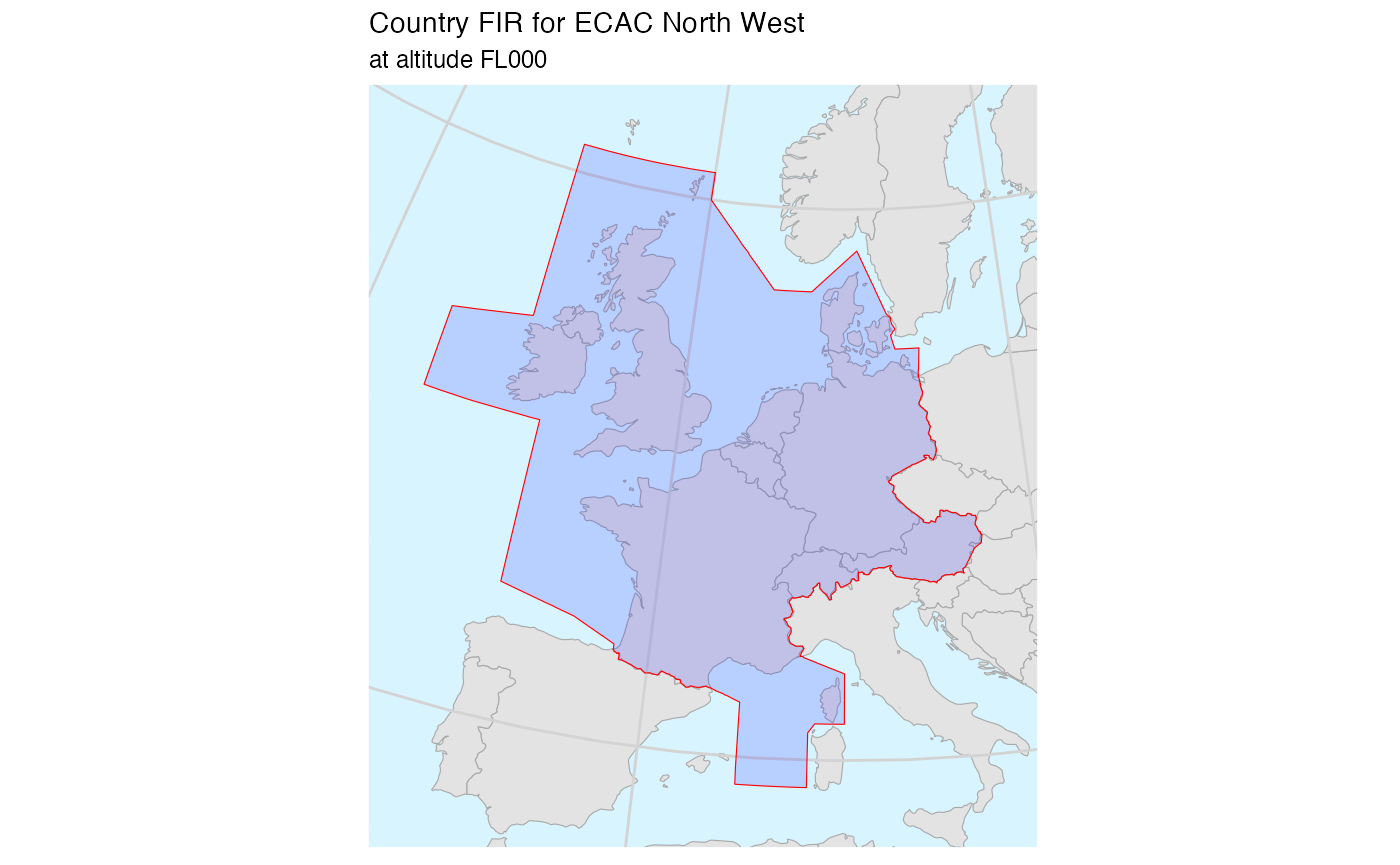
ECAC South West
ecac_southwest() %>%
  plot_country_fir(icao_id = "ECSW",
                   name = "ECAC South West",
                   firs = .)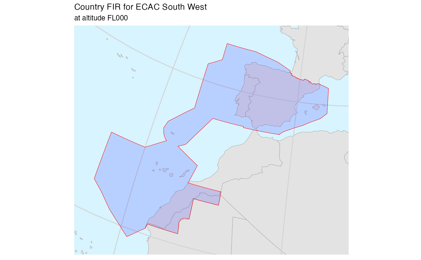
ECAC North East
ecac_northeast() %>%
  plot_country_fir(icao_id = "ECNE",
                   name = "ECAC North East",
                   firs = .)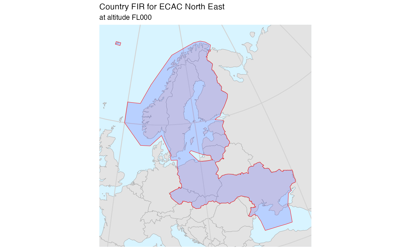
ECAC South East
ecac_southeast() %>%
  plot_country_fir(icao_id = "ECSE",
                   name = "ECAC South East",
                   firs = .)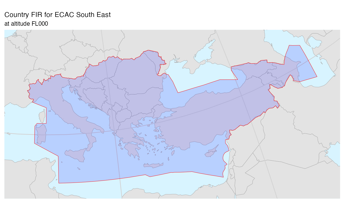
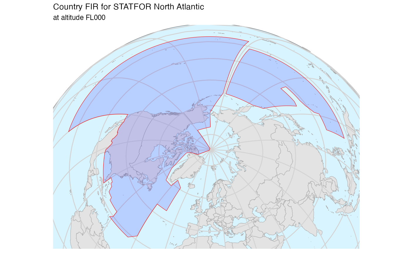
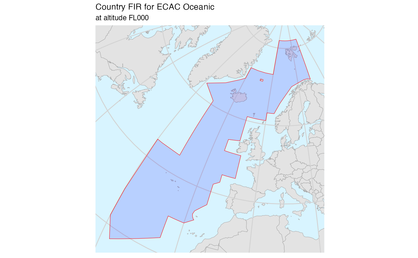
North Atlantic
st_segmentize improved things but THIS IS still BAD!
firs <- system.file("extdata", "icao_firs.geojson", package = "pruatlas") %>%
  read_sf() %>%
  rename(icao = icao_code)
north_atlantic() %>%
  sf::st_segmentize(dfMaxLength = units::set_units(50, km)) %>%
  plot_country_fir(icao_id = "NOAT",
                   name = "STATFOR North Atlantic",
                   firs = .)